The original post was supposed to be about gradient boosted decision trees. But before delving into this, I realized that a quick post on decision trees might be helpful. This post is a bit different from the others as it will mostly comment a simplified version of the implementation of decision trees developed by the numpy-ml package.
Introduction & Motivation
As scikit learn puts it decision trees (DTs) are a “non-parametric supervised learning method used for classification and regression”. One of the main advantages of decision trees it that we can understand and interpret them. One disadvantage is that the trees might be overfitting loosing generalizability.
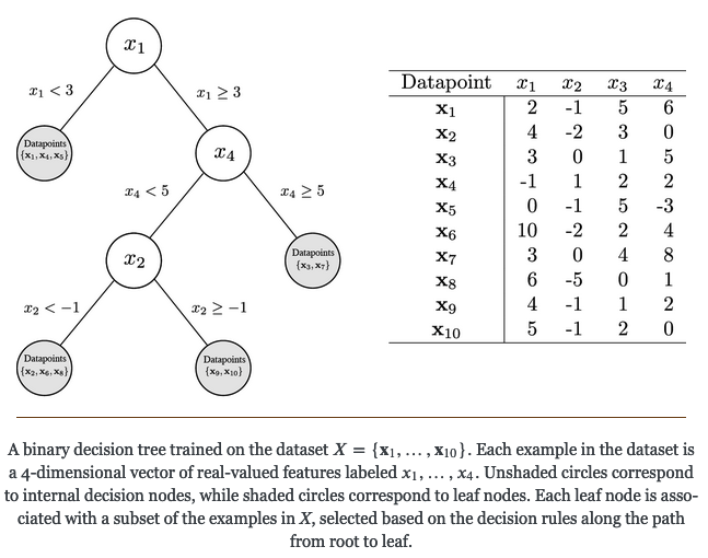
The image below from the numpy-ml package provides a high level overview on decision trees:
Evaluation Criteria
Generally, there exist two criteria that used to evaluate whether to go further down the tree or to stop:
-
Information Entropy: $-\sum_j P_n(\omega_j) \log P_n(\omega_j)$ where $P_n(\omega_j)$ is the fraction of data points at split $n$ associated with $\omega_j$
-
Gini Impurity: $\sum_{i \neq j} P_n(\omega_i) P_n(\omega_j) = 1 - \sum_{j} P_n(\omega_j)^2$
Let’s put these two into Python functions. I follow the numpy-ml package here:
def entropy(y):
    """
    Information Entropy
    """
    hist = np.bincount(y)
    ps = hist / np.sum(hist)
    return -np.sum([p * np.log2(p) for p in ps if p > 0])


def gini(y):
    """
    Gini Impurity
    """
    hist = np.bincount(y)
    N = np.sum(hist)
    return 1 - sum([(i / N) ** 2 for i in hist])
Implementation
Fit
Now, let’s follow the numpy-ml package step by step and evaluate the code bits. On a high level we have the fit and predict functions. The fit function learns on the data and the predict function gives us the predictions depending on the input data we provide it with. Let’s start with the fit() function.
def fit(self, X, Y):
    """
    Fit a binary decision tree to a dataset.
    Parameters
    """
    # determine how many features we consider for each splits (n_feats)
    self.n_feats = X.shape[1]
    self.root = self._grow(X, Y)
Here, we only determine how many features we would like to consider for each split (n_feats). For illustration purposes here it is set to all. Then reference is made to _grow(). _grow() first checks if the Y values do vary because not we already found a solution. Then a random sample of the number of columns in the $X$ variables is created with the size of the number of features we consider (np.random.choice(M, size = self.n_feats, replace = False)). The randomness is actually only relevant if we do not consider all features, so in our case this can be ignored. These numbers are then fed into the _segment() function to determine the best split. That is then repeated by calling _grow() again on the next level of the tree.
def _grow(self, X, Y, cur_depth=0):
        # if all labels are the same, return a leaf
        if len(set(Y)) == 1:
            return Leaf(Y[0])

        # if we have reached max_depth, return a leaf
        if cur_depth >= self.max_depth:
            v = np.mean(Y, axis=0)
            return Leaf(v)

        cur_depth += 1
        self.depth = max(self.depth, cur_depth)

        N, M = X.shape

        # generate a random sample from the 1-D array of M columns without replacement
        feat_idxs = np.random.choice(M, size = self.n_feats, replace = False)

        # greedily select the best split according to `criterion`
        # apply segment function
        feat, thresh = self._segment(X, Y, feat_idxs)
        l = np.argwhere(X[:, feat] <= thresh).flatten()
        r = np.argwhere(X[:, feat] > thresh).flatten()

        # grow the children that result from the split
        left = self._grow(X[l, :], Y[l], cur_depth)
        right = self._grow(X[r, :], Y[r], cur_depth)
        return Node(left, right, (feat, thresh))
Now what does _segment() do? _segment() goes through each of the split columns (i.e. all columns in our case) that we provided the function with and evaluates for each of the columns at different thresholds what the impurity gain would be. This is measured with the _impurity_gain() function which gathers for each threshold the impurity gain. Then finally the threshold for the maximum impurity gain is saved.
def _segment(self, X, Y, feat_idxs):
    """
    Find the optimal split rule (feature index and split threshold) for the
    data according to `self.criterion`.
    """
    best_gain = -np.inf
    split_idx, split_thresh = None, None
    for i in feat_idxs:
        # get the i-th column which we created before with the number generator
        vals = X[:, i]
        levels = np.unique(vals)
        # [:-1] -> take all but the last element
        # [1:] -> take all but the first element
        thresholds = (levels[:-1] + levels[1:]) / 2 if len(levels) > 1 else levels
        # now call function impurity gain
        # collect all values of the gain in list (for each threshold)
        gains = np.array([self._impurity_gain(Y, t, vals) for t in thresholds])

        # update the gain if new one is btter
        if gains.max() > best_gain:
            split_idx = i
            best_gain = gains.max()
            # save the threshold for the max gain
            split_thresh = thresholds[gains.argmax()]

    return split_idx, split_thresh
Keep in mind that we want to maximize the reduction in impurity. So what does the _impurity_gain() function do?
First of all, we opt for one of the loss functions determined earlier (e.g. entropy, gini). Second, the loss of the parent split is calculated. Third the row indices of the of the splits proposed by the threshold that we input are obtained (np.argwhere(feat_values <= split_thresh).flatten()). With these indices the losses (e.g. entropy loss provides negative result) for the two groups (Y left, Y right) are calculated (= child loss). And then a weighted average of the two losses is taken. Finally, the impurity gain is calculated as the parent loss minus the child loss and this is then returned.
    def _impurity_gain(self, Y, split_thresh, feat_values):
        """
        Compute the impurity gain associated with a given split.
        IG(split) = loss(parent) - weighted_avg[loss(left_child), loss(right_child)]
        """
        if self.criterion == "entropy":
            loss = entropy
        elif self.criterion == "gini":
            loss = gini

        # calculate the loss of the parent before the split
        parent_loss = loss(Y)

        # generate splits by getting all index positions where the value is <= or > than the threshold
        left = np.argwhere(feat_values <= split_thresh).flatten()
        right = np.argwhere(feat_values > split_thresh).flatten()

        if len(left) == 0 or len(right) == 0:
            return 0

        # compute the weighted avg. of the loss for the children
        n = len(Y)
        # number of indices making the threshold
        n_l, n_r = len(left), len(right)

        # calculate loss according evaluation criterion defined
        # taking the rows by left and right index of Y as the input
        e_l, e_r = loss(Y[left]), loss(Y[right])
        child_loss = (n_l / n) * e_l + (n_r / n) * e_r

        # impurity gain is difference in loss before vs. after split
        ig = parent_loss - child_loss
        return ig
In the end, _grow() saves the results in the Node class:
class Node:
    def __init__(self, left, right, rule):
        self.left = left
        self.right = right
        self.feature = rule[0]
        self.threshold = rule[1]
The end values are saved in the Leaf() class.
class Leaf:
def __init__(self, value):
    """
    `value` is an array of class probabilities if classifier is True, else
    the mean of the region
    """
    self.value = value
Predict
Now, after the training (fit) we can focus on the prediction where we traverse the trained decision tree for each x value that is encountered.
def predict(self, X):
    """
    Use the trained decision tree to classify or predict the examples in `X`.
    """
    # iterates over rows of X!
    return np.array([self._traverse(x, self.root) for x in X])
Here the _traverse function becomes in important. First it checks whether the root is a leaf. If this is not the case the function checks whether the x value at the column position is smaller or equal to the node’s threshold. If this is the case the tree is traversed again. This recursive procedure is repeated until the end of the tree is reached.c
def _traverse(self, X, node, prob=False):
    if isinstance(node, Leaf):
        return node.value
    if X[node.feature] <= node.threshold:
        return self._traverse(X, node.left, prob)
    return self._traverse(X, node.right, prob)
Now, let’s test this out:
dt = DecisionTree()
X = np.array([[2,-1,5,6],[4,-2,3,0],[3,0,1,5], [-1,1,2,2]])
Y = np.random.choice(10,4)
dt.fit(X,Y)
dt.predict(X)
Hope this was illustrative.
Sources
- Bourgin, D. numpy-ml. (2022).
- Breiman, L., Friedman, J. H., Olshen, R. A. & Stone, C. J. Classification and regression trees. Wadsworth. Inc. Monterey, California, USA (1984).
- Lanaro, G. Implementing Decision Trees in Python. https://gabrielelanaro.github.io/blog/2016/03/03/decision-trees.html.